If you’d prefer to watch the full video, please click below!
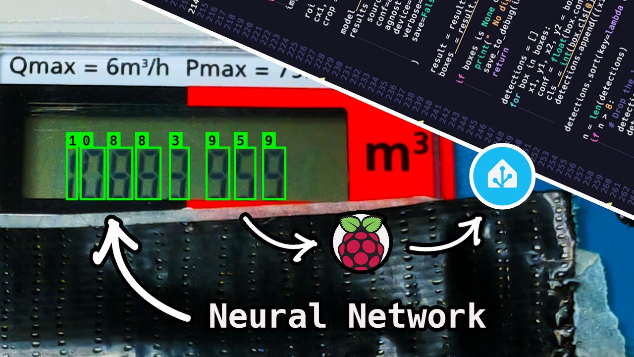
Every month, I have to crawl into a cupboard under my stairs, point a torch at my gas meter, and read off eight tiny digits to send to my energy supplier. So I did the only reasonable thing: I put a camera in the cupboard and taught a computer to do it for me.
In this post I’ll take you the whole way — and it’s a proper walkthrough, not just a tour. You’ll see how I built the rig that watches the meter, how a computer actually sees an image, then the exact commands to label your photos, train the model, and run it yourself, how it talks to Home Assistant, and finally how it automatically submits the reading to the gas company so I never have to crawl in there again. All the code is on GitHub if you want to follow along.
What You’ll Need
Let’s start with the hardware. The whole capture rig is deliberately simple.
Core Components
Raspberry Pi 4 – This is what we’ll run the model on - though, any raspberry pi from 3+ should also work.
Raspberry Pi Camera Module 3 – Captures our meter images.
A small light source – Consistent light dramatically improves the images (and the readings).
Patience – The single most important ingredient. You need to collect thousands of photos before any of this works.
Step 1: Build the Capture Rig
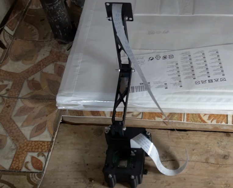
I wedged the Pi and camera into the cupboard, pointed it at the display, and that was the whole rig. The software side is a single cron job that fires every 10 minutes:
Take a photo with the rpicam-jpeg tool.
Rotate it 180° (the camera is mounted upside-down).
Apply a region-of-interest (ROI) crop so I’m only keeping the slice of the frame the meter lives in.
Stamp it with the date and save it to a folder.
#!/usr/bin/env bashset-euo pipefail
SAVE_DIR="/home/pi/meter-captures"mkdir-p"$SAVE_DIR"DATETIME=$(date +"%Y%m%d_%H%M%S")
rpicam-jpeg --rotation 180 --roi 0.25,0.20,0.5,0.5 -o"${SAVE_DIR}/${DATETIME}.jpeg"# This will come later. For now, you can focus on above
python3 /home/pi/meter-ocr/infer_yolo.py \--model /home/pi/meter-ocr/model_digit_yolo.onnx \"${SAVE_DIR}/${DATETIME}.jpeg"echo"Files in '$SAVE_DIR':"
find "$SAVE_DIR"-maxdepth 1 -type f -printf" %TY-%Tm-%Td %TH:%TM %f\n" | sort
echo""echo"Deleting files older than 1 day..."
find "$SAVE_DIR"-maxdepth 1 -type f -mtime +1 -print-deleteecho"Done."
# /etc/cron.d/gas-capture — fires every 10 minutes*/10 **** pi /home/pi/meter-ocr/capture.sh
Then I just let it run. For weeks… We’ll need these later on to train our model.
This is the tedious truth about machine learning: before you can do anything meaningful, you have to collect the data. That growing folder of photos is the single most important ingredient in the whole project. Every so often, I rsync‘d the pile back to my laptop to add to the training set.
Step 2: Understand How a Computer “Sees”
Before training anything, it’s worth understanding what the model is actually working with — because it’s not a picture.
To a computer, an image is a grid of pixels, and each pixel is just three numbers: how much red, how much green, and how much blue, from 0 to 255. There are no shapes, no digits — just numbers.
If you collapse those three values down to one (pure brightness) and lay them out on a grid, the digit is suddenly right there, hiding in the numbers. High values where the segment glows, low where it’s dark.
So how does a computer find a pattern in a wall of numbers? It slides a small window — called a filter or kernel — across the image. At every position, it multiplies each number underneath by the matching number in the kernel, adds them up, and writes out a single value. Sweep that across the whole image and you’ve measured one specific thing everywhere at once — “is there a sharp edge here?”
That sweep produces a new grid called a feature map: bright where the pattern is strong, dark where it’s weak. Stack hundreds of these, each hunting a different pattern, and that pile of matrices is what the network actually works on. Not pixels, not pictures — numbers, all the way down.
Step 3: How the Network Works
Rather than build a model from scratch, we’ll use YOLO (You Only Look Once), a well-known object detector, and supplemented it with my own gas-meter photos so it learned my display.
Step 4: Label the Data and Train the Model
Everything from here runs on your laptop, not the Pi. All the code is in the smart-gas-meter repo — grab it and set up a virtual environment:
Now you need some photos in data/meter-captures/. If you collected your own on a Pi, copy them over (there’s a sync_captures.sh helper that pulls them via SCP). If you’d rather just follow along, I’ve published my full set of ~3,200 captures on Hugging Face — grab and unzip it into data/:
The dataset is Cian911/meter-captures (CC-BY-4.0), so you can label and train on exactly the images I used.
Calibrate the crop (one time)
The scripts need to know where on the frame your display sits. Run the one-time calibration — it pops up an image, you draw a box around the LCD, then click the left edge of each digit. It writes those bounds to roi_config.json:
extract.py walks through every capture in data/meter-captures/, crops out the display region using your calibration, and writes greyscale crops to data/extracted/. Two small things happen to each crop. First, it’s run through CLAHE (contrast-limited adaptive histogram equalisation) — this evens out the lighting so a digit looks the same at 8am as it does at 3pm:
Second, it sanity-checks the crop by mean brightness. If the display is obstructed or blown out by glare, the average pixel value falls outside a sensible band and the frame gets flagged so you can go look at it:
python extract.py
# → Done: 3180 good, 49 flagged out of 3229 images.# → Display crops saved to data/extracted/
Label the crops
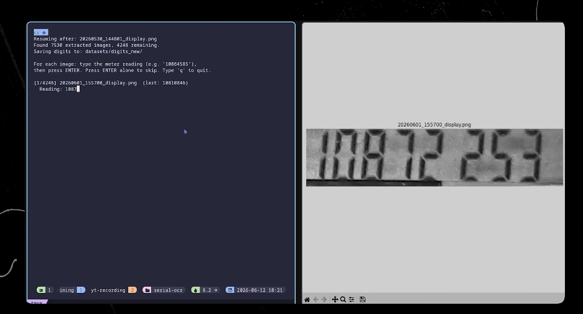
Before any training, every photo needs the right answer attached — a photo on its own teaches the model nothing. label.py flashes each crop on screen and waits for you to type the reading. The loop is basically this: show the crop, read what you type, validate it’s digits, and save your progress immediately:
reading=input(prompt).strip()ifreading.lower()=="q":print("Quitting.")breakifnotreading:# ENTER alone → skip a blurry one
progress[fname]="skipped"save_progress(progress)continue# ... crop into per-digit images, then record the answer
progress[fname]=readingsave_progress(progress)# saved after every entry — quit any time
Because it saves after every single entry to label_progress.json, you can stop and pick up exactly where you left off:
I did this more than three thousand times across a few evenings. After throwing out the blurry and half-captured frames, I was left with 3,229 clean, fully-labelled photos, all recorded in label_progress.json.
Build the training set
prepare_yolo_dataset.py turns that label file into the format YOLO expects — images plus a text file of bounding boxes per image — and does the train/validation split for you.
Here’s the one clever bit in the data prep: it does not crop tightly to the display. It adds 300 pixels of padding on every side. Why? Because I want the model to learn “the digits are somewhere in this wide band” — not “the digits are at these exact pixels.” That padding is camera-drift insurance: the camera can shift a few centimetres and the model still finds the digits, no recalibration needed. You can see it right in the crop bounds:
PADDING=300defget_crop_bounds(img_w,img_h,roi):"""Loose crop around the display ROI, clamped to image bounds."""rx,ry,rw,rh=roi["x"],roi["y"],roi["w"],roi["h"]cx1=max(0,rx-PADDING)cy1=max(0,ry-PADDING)cx2=min(img_w,rx+rw+PADDING)cy2=min(img_h,ry+rh+PADDING)returncx1,cy1,cx2,cy2
Then it shuffles everything with a fixed seed (so the split is reproducible) and holds back 20% for validation — the photos the model never trains on:
Now the actual fine-tuning. I did not train this from scratch — I couldn’t. A network with 3.2 million parameters, starting from random noise, needs millions of images just to learn what an edge is. I had a few thousand photos of one meter in a cupboard.
The trick is transfer learning. train_yolo.py starts from yolov8n.pt — a YOLOv8-nano model already trained on around 120,000 everyday photos. It already knows what edges, curves, and shapes look like. It just keeps training on your meter photos — this is called fine-tuning. Nothing is frozen; the whole network keeps learning, but it starts from “understands images” instead of “random noise”, and only has to re-aim that knowledge at one job: find digits.
The whole thing is one train() call. Loading yolov8n.pt as the base is what makes it transfer learning; patience=15 is the early-stop — if 15 epochs pass with no improvement, it stops rather than grinding away:
model=YOLO(args.model)# args.model defaults to "yolov8n.pt"
results=model.train(data=str(DATASET_YAML),epochs=args.epochs,# up to 100
batch=args.batch,# 16
imgsz=args.imgsz,# 640
patience=15,# early-stop after 15 epochs with no gain
)
Training itself is just a loop: the model guesses where the digits are, checks how wrong it was (that error is the loss), and nudges its millions of parameters a touch to be less wrong next time. Do that over and over and the loss slides down while accuracy climbs. Kick it off:
On a laptop GPU that’s about an hour, and it’s usually over 99% accurate within a few epochs.
The Honest Test
I graded the model only on the 20% it had never seen, so I’m measuring whether it actually learned to read meters — not whether it memorised my training pile. The results:
Metric
Score
mAP@50
≈ 0.995
Precision
≈ 0.9995
Recall
≈ 1.0
On photos it had never seen before, it finds every single digit, basically every time, and almost never gets one wrong. For reading a gas meter, you genuinely can’t ask for much more than that.
Step 5: Run It
With a trained model, you can read any capture from the command line. infer_yolo.py takes an image, applies the same 300px-padded crop the model trained on, and runs the detector. What comes back is a bag of boxes in no particular order — this is the decode step from Step 3, in real code. Sort the detections left-to-right by their x-centre, and the reading falls out:
detections.sort(key=lambdad:d[0])# d[0] is the box x-centre
digit_str="".join(str(d[1])fordindetections)# d[1] is the class 0–9
reading=format_reading(digit_str)# "10872253" → "10872.253"
A meter has exactly 8 digits, so anything else is wrong by definition — too many detections (a reflection read as a 9th digit), drop the least confident; too few, bin the frame:
n=len(detections)ifn>8:# keep the 8 most-confident, then re-sort left-to-right
detections=sorted(detections,key=lambdad:d[2],reverse=True)[:8]detections.sort(key=lambdad:d[0])elifn<8:print(f" Expected 8 digits, got {n} — skipping.")return
--debug also saves an annotated crop with the green boxes drawn on, so you can see what it found:
That’s the whole thing working on your laptop. The last job is getting it onto the Pi so it runs by itself.
Deploying to the Pi
The model trained on my laptop with a GPU, but the thing that has to run every 10 minutes is Raspberry Pi. Getting a model to actually run on the Pi takes a bit of fiddling. It runs best in a format called ONNX — a portable, Pi-friendly version of the model. (Running the raw PyTorch model on the Pi gives you an Illegal instruction crash; the DEPLOYMENT.md guide covers exactly why and the gotchas.) A single inference takes roughly 300–500ms on the Pi.
Export the trained weights to ONNX, then copy the model, the inference script and your calibration over:
# On your laptop — export to ONNX
python -c"from ultralytics import YOLO; YOLO('model_digit_yolo.pt').export(format='onnx', imgsz=640, simplify=True)"# Copy to the Pi
scp infer_yolo.py model_digit_yolo.onnx roi_config.json pi@raspberrypi.local:/home/pi/meter-ocr/
# On the Pi — install the runtime (no PyTorch needed)
pip install ultralytics onnxruntime opencv-python-headless python-dotenv
Now the capture job from Step 1 gets its extra step back — the infer_yolo.py line I told you to ignore earlier. Every 10 minutes the Pi snaps the photo, runs the ONNX model, and produces a reading in well under a second — right there in the cupboard, in the dark, pointing at the model with --model model_digit_yolo.onnx.
Reporting to Home Assistant
A number sitting on a Pi isn’t much use, though — I want it in my smart home. I run Home Assistant, so I generated a long-lived access token (basically a permanent password for the script). Copy .env.example to .env on the Pi and drop your details in:
That state_class: total_increasing tag is the important one — it tells Home Assistant this is a value that only ever counts up, which is exactly what lets the Energy dashboard chart my actual gas use over time. Add it under Settings → Energy → Gas consumption and you get a live gas-meter card and a full consumption history, built entirely from a camera and a model you trained on your own photos.
Guardrails: Don’t Trust the Model Blindly
A model that’s right 99.5% of the time is still wrong sometimes, and one bad reading can poison the whole graph. So nothing gets posted until it clears two checks:
Confidence gate – If the model’s mean confidence is below 0.80, it doesn’t post; it just flags the photo for me to review.
Physics gate – A gas meter can only go up, and it can’t realistically jump more than a tiny amount in 10 minutes. So if a reading goes backwards, or leaps up too far, I know the model misread a digit and I bin it.
That second, common-sense rule catches mistakes that confidence alone never would — and it’s barely any code:
MAX_READING_JUMP=2.0# max plausible m³ increase between readings
defis_plausible(reading_str,prev):value=float(reading_str)ifprevisNone:returnTrue,"no prior reading"ifvalue<prev:returnFalse,f"{value} is lower than last known {prev:.3f} (meters never go backwards)"ifvalue-prev>MAX_READING_JUMP:returnFalse,f"jump of {value-prev:.3f} m³ exceeds MAX_READING_JUMP={MAX_READING_JUMP}"returnTrue,"ok"
Step 6: Auto-Submit to the Gas Company
The original goal was never having to crawl into that cupboard again — and that means the reading has to go one step further, to the gas company itself.
Here in Ireland, Gas Networks Ireland take readings through an online form. And a web form is just an HTTP POST under the hood: you need the gprn number (your meter’s ID), the reading, and a couple of other form fields. submit_gni.py handles the whole round-trip — always try it with --dry-run first, which scrapes the form and prints the payload without submitting:
# Dry run — print the payload, do NOT submit
python submit_gni.py --dry-run--gprn 0124793 10883
# Real submit (decimal is dropped automatically → 10883)
python submit_gni.py --gprn 0124793 10883.253
There are a couple of real-world quirks the script deals with for you: Gas Networks Ireland only accept one reading per GPRN every 14 days (it tracks this locally so it won’t waste a network call), the form’s hidden form_build_id token changes on every page load, and it only wants the whole-m³ integer part. All of that is handled — you just give it a reading.
Here’s the full chain, working end to end: once a reading clears both gates, then on the right day of the month, the Pi fires it straight at the provider and logs the confirmation it gets back. No human in the loop. A meter that reads itself, sanity-checks itself, and files its own returns.
Real-World Problems (Because Nothing Works First Try)
None of this worked on the first attempt. The interesting part is what broke:
Light. The same meter looks completely different at 8am versus 3pm. My very first attempt used hand-written rules and contrast tricks — it would work all week and then fall apart on a sunny Tuesday afternoon. That fragile pipeline is the entire reason I switched to a detector that just learns the lighting from thousands of examples.
Camera drift. Every time I bumped the cupboard door, the camera shifted a hair. With tight cropping, that was fatal — the crop sliced the wrong pixels. The 300px padding from Step 4 made drift stop mattering entirely.
Too many digits. A glare or reflection would occasionally make the model see a ninth digit; a blurry frame would give only seven. The display has exactly 8 digits, so I normalise to 8: too many, drop the least-confident extras; too few, bin the image.
Wrapping Up
So that’s the journey. We built a camera into a cupboard and let it pile up thousands of photos. We learned that to a computer, an image is just a wall of numbers. We slid filters over it to find patterns and stacked those into a network. We didn’t build it from scratch — we stood on a model that already understood the visual world and fine-tuned it for one job. Then we put the trained brain back into that 5-watt computer in the cupboard, taught it to talk to Home Assistant, and bolted on guardrails so it never lies to me.
The thing I keep coming back to: my first version had five fiddly preprocessing steps and still broke on sunny afternoons. This version has one real step — feed the image in, get the reading out. When your preprocessing gets complicated, it usually means you’re fighting the data. Let the model do the fighting, and a lot of the pain just disappears.
If you enjoyed this, be sure to share this article or subscribe on YouTube for more machine learning and DIY smart home projects. Got questions or ideas for what I should point a camera at next? Drop them in the comments.
Turning a Singing Fish into a Smart AI Assistant with ESP32 and Home Assistant
Bring your Billy Bass back to life with AI! Learn how to turn a singing fish into a fully interactive smart assistant using ESP32-S3, ESPHome, and Home Assistant’s Summer of AI features. Includes custom wake word, real-time mouth motion, and OpenAI-powered conversations.
How to Build an ESP8266 Infrared Smart Controller for Home Assistant
Turn your old infrared-controlled devices into smart home gadgets! This step-by-step guide shows you how to build an ESP8266 IR controller that can both receive and send signals, integrate with Home Assistant or Alexa, and stay in sync with your original remote. Includes full wiring, ESPHome YAML, and testing walkthroughs.